SAS Macro Programs for Statistical Graphics: LOWESS
$Version: 2.2 (21 Dec 2003)
Michael Friendly
York University
The LOWESS macro performs robust, locally weighted scatterplot
smoothing as described in "Section
4.4.2". The data and the smoothed curve are plotted if
PLOT=YES is specified. The smoothed response variable, residuals,
and observation weights are returned
in the output data set named by the OUT= parameter.
An optional output ANNOTATE= data set can also be produced, which may be used
to apply the lowess smoothing in a more complex plotting application.
As of Version 2.1, the LOWESS macro will use PROC LOESS if running under
Version 7 of the SAS System.
This makes the macro much faster, particularly for large data sets.
For use with SAS 6.12 or earlier, use the STEP= parameter to control
the number of data points at which the local regressions are computed.
Parameters
- DATA=_LAST_
- Name of the input data set.
- X = X
- Name of the independent (X) variable.
- Y = Y
- Name of the dependent (Y) variable to be
smoothed.
- ID=
- Name of an optional character variable to
identify observations.
- OUT=SMOOTH
- Name of the output data set. The output
data set contains the X=, Y=, and ID= variables
plus the variables _YHAT_, _RESID_, and
_WEIGHT_. _YHAT_ is the smoothed value of the
Y= variable, _RESID_ is the residual, and
_WEIGHT_ is the combined weight for that
observation in the final iteration.
- F = .50
- Lowess window width, the fraction of the
observtions used in each locally-weighted
regression. A larger window width makes the
curve smoother, but may lead to lack of fit.
Values of F > 1 are allowed.
- P = 1
- Degree of the locally-weighted regressions.
P=1 gives linear fits, appropriate when the
data do not have several peaks and valleys; P=2
gives quadratic fits, which are useful when
they do.
- ITER=2
- Total number of iterations.
- ROBUST=1
- Specifies whether to perform robustness re-weightings,
which decrease the weights for observations with large residuals in the
next iteration. Set ROBUST=0 to suppress the robust calculations.
For binary dependent variables, the robustness step is usually not
performed.
- CLM=
- [Version 7+ only]
Specifies the significance level for confidence intervals about the
smoothed curve. Use CLM=0.05 for 95% confidence intervals.
- STEP=1
- Step for successive X values. By default, the
macro performs the locally-weighted regression at each X[i], which
can be computationally intensive for moderately large data sets.
Setting STEP > 1 causes the macro to perform the regression at
every STEP-th value of the index i, and to use predicted values from
that regression for intermediate points. It is recommended to specify
a STEP value at least n/100 for moderate to large sized datasets.
- PLOT=NO
- Specifying PLOT=YES, draws both a printer plot and a
high-resolution plot. You may wish to change the
default values of the PLOT, GPLOT or PPLOT options to suit your taste.
- GPLOT=NO
- Draw the plot? If you specify PLOT=YES, a
high-resolution plot is drawn by the macro.
- PPLOT=NO
- Draw a printer plot? If you specify
PPLOT=YES, a printer plot is drawn by the
macro.
- SYMBOL=CIRCLE
- Plotting symbol used for points
- HTEXT=1.5
- Height for axis labels and values
- HSYM=1.5
- Height for point symbols
- COLORS=BLACK RED
- colors for points and smooth curve
- LINE=1
- Line style for the smooth curve
- HAXIS=
- The name of an AXIS statements for the horizontal axis
- VAXIS=
- The name of an AXIS statements for the vertical axis
- OUTANNO=
- Name of output ANNOTATE= dataset which draws the
smoothed lowess curve. This dataset is produced only if the OUTANNO=
name is specified.
- IN=
- Name of an optional input ANNOTATE= data set,
which is concatenated to the OUTANNO= data set.
- NAME=LOWESS
- The name assigned to the graph in the
graphic catalog.
Missing data
Any observations with missing data on the X or Y variables are
removed before finding the lowess fit.
Usage Note
Under some older versions of the SAS System,
it may be neccessary to add the option WORKSIZE=100 to
the PROC IML statement.
Example
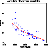
This example plots gas mileage (MPG) vs weight, with a smoothed lowess
curve showing a (slight) nonlinear dependence of mileage on weight.
The plot is drawn by the macro from the OUT=SMOOTH data set.
An output ANNOTATE= data set is also produced.
title 'Auto data with lowess smoothing';
%include data(auto);
%include macros(lowess);

%lowess(data=auto,out=smooth, x=weight, y=mpg,
    id=model, htext=2,
    f=.4, plot=YES,
    colors=blue red, outanno=lowess);

