faces Faces display of multivariate data faces

SAS Macro Programs: faces

$Version: 1.6-0 (28 Sep 2011)
Michael Friendly
York University


The faces macro ([download] get faces.sas) ([download] get facekey.sas)

Faces display of multivariate data

The faces macro draws (possibly) asymmetric faces to represent multivariate data, mapping the values of variables into parameters that control the size, orientation, and location of facial features.

The display is organized into one or more rectangular "blocks" per page; each block may have any number of rows and columns.

Note: The program generates a very large data set to draw the faces, approximately 800 annotate observations for each face. Disk usage depends on the number of faces plotted per page, which is the product of the parameters BLKS * ROWS * COLS. The RES option controls the number of plotting observations for each face.

The FACEKEY macro creates a legend for a faces display showing the assignment of variables to facial features.

Method

The use of faces to display multivariate data was suggested by Chernoff (1973). Flury and Reidwyl (1981) developed the method for asymmetric faces, and for parameterizing each facial feature by coeficients of a 5-th degreee polynomial whose values could be assigned to data variables. The current faces macro program is based on an earlier version by M. Schupach (1989).

Facial parameters

There are 18 parameters of a face which may be assigned to variables in the data set. The parameters may be assigned to the same variables for both the left and right sides of the face, giving symmetric faces, or they may be assigned to different variables for the left and right sides, giving asymmetric faces.

Each parameter normally ranges from 0 to 1. It is the user's responsibility to scale the data appropriately before calling FACES. (See the scale macro for this.). Alternatively, the option STD=RANGE may now be used to perform this scaling internally.


Parameter Facial Feature
1 (EYSI) Eye size
2 (PUSI) Pupil size
3 (POPU) Position of pupil
4 (EYSL) Eye slant
5 (HPEY) Horizontal position of eye
6 (VPEY) Vertical position of eye
7 (CUEB) Curvature of eyebrow
8 (DEEB) Density of eyebrow
9 (HPEB) Horizontal position of eyebrow
10 (VPEB) Vertical position of eyebrow
11 (UPHA) Upper hair line
12 (LOHA) Lower hair line
13 (FALI) Face line
14 (DAHA) Darkness of hair
15 (HSSL) Hair shading slant angle
16 (NOSE) Nose line
17 (SIMO) Size of mouth
18 (CUMO) Curvature of mouth

Usage

faces is a macro program. You should specify the assignment of variables to facial features using either the LEFT= and RIGHT= parameters, or using the parameters L1=, L2=, ...,L18=, R1=, R2=,... R18=. The individual Ln= and Rn= parameters take precedence if a feature appears in both sets of parameters.

The arguments may be listed within parentheses in any order, separated by commas. For example:

   %faces(left=variables, right=variables, ..., )

Parameters

DATA=_LAST_
The name of the input dataset. If not specified, the most recently created dataset is used.
LEFT=
List of names of (up to) 18 variables to be assigned to features of the left side of the face.
RIGHT=
R1= R2= R3= R4= R5= R6= R7= R8= R9= R10= R11= R12= R13= R14= R15= R16= R17= R18=
L1= L2= L3= L4= L5= L6= L7= L8= L9= L10= L11= L12= L13= L14= L15= L16= L17= L18=
Variables can be assigned to features either by listing 18 variable names for LEFT and RIGHT or by assigning individually to Ln and Rn parameters. Variable names can appear more than once. Use . in LEFT= or RIGHT= to skip a parameter (leaving it unassigned). The variables are each assumed to have been pre-scaled to the interval (0, 1), unless STD=RANGE is used..
OUT=ASYM
Name of output Annotate data set
ID=
Name of a character ID variable used to label the plot cell for a given observation.
IDNUM=
Name of a numeric ID variable. Default: observation number
STD=
Specify STD=RANGE to standardize the variables internally to a range of (0, 1).
MIN=.
Specify a non-missing value to enforce/allow a minimum scaled value different from 0. Use this option with caution.
MAX=.
Specify a non-missing value to enforce/allow maximum scaled value different from 1. Use this option with caution.
BLKS=1
Blocks per page
ROWS=4
Rows per block
COLS=4
Columns per block
RES=3
Resolution: 1=high/3=low. Higher resolution means more lines are drawn for each facial feature.
FRAME=Y
Draw a frame around each face? Y or N.
COLOR='BLACK'
Color of each face. Specify a variable name or a string in quotes. If a variable name is specified, the values are assumed to be color names.
HCOLOR='BLACK'
Hair color. Specify a variable name, or a string in quotes.
ECOLOR='BLACK'
Eye color. Specify a variable name, or a string in quotes.
ROW=
The name of an optional variable whose value indicates which row in a block an observation is drawn in. The ROW=, COL=, and BLK= parameters may be used to assign particular locations to faces. Otherwise, the faces are drawn in the order of observations in the data set.
COL=
The name of an optional variable whose value indicates which column in a block an observation is drawn in.
BLK=
Names of variables indicating the row, column, and block in which the face for a given observation is to be drawn.
GOUT=GSEG
Name of graphics catalog in which the plot is stored
NAME=FACES
Name for graphic catalog entry

Missing data

Any missing variables for an observation are replaced by 0.5.

Example

This example plots faces to represent the mean of cars in the auto dataset, classified by region of origin. An initial datastep is used to align the scales of all variables so that large values represent 'better' cars. Then, all variables must be scaled to a range of 0-1.
%include macros(faces);        *-- or include in an autocall library;
%include macros(scale) ;
%include data(autom)  ;
goptions vsize=7.5 hsize=7.5in  lfactor=4;
title h=1.8 "Faces Plot of Automobile data";
 
data autom;
   length clr $8;
   set autom;
   if rep77 ^= . and rep78 ^=.;       /* delete missing data         */
   if rep78 =. then rep78=rep77;
   price = -price;                  /* change signs so that large  */
   turn  = -turn;                   /* values represent 'good' cars*/
   gratio= -gratio;
   weight=-weight;
   length=-length;
   select;
      when (origin ='A')  clr = 'RED';
      when (origin ='E')  clr = 'GREEN';
      when (origin ='J')  clr = 'BLUE';
      otherwise clr='BLACK';
   end;

%scale(data=autom,
       out=scaled,
       outstat=range,
       var = gratio  turn  rep77  rep78  price    mpg
            hroom rseat  trunk weight length displa,
       copy=clr _freq_,
       id=id);
data scaled;
   set scaled;
	where id in ('Average', 'American', 'European', 'Japanese');
run;
The faces macro is called as follows. Note that although there are only 4 faces, to display them in one row, without distortion, the ROWS parameter is set to 4.
%faces(data=scaled,
       id=id,    idnum=_freq_,      color=clr,
       res=3,
       blks=1, rows=4, cols=4,
       l1 =mpg,      r1 =mpg,
       l2 =mpg,      r2 =mpg,
       l3 =turn,     r3 =turn,
       l4 =turn,     r4 =turn,
       l5 =hroom,    r5 =hroom,
       l6 =hroom,    r6 =hroom,
       l7 =rseat,    r7 =trunk,
       l8 =rseat,    r8 =trunk,
       l9 =displa,   r9 =displa,
       l10=length,   r10=length,
       l11=rep77,    r11=rep78,
       l12=weight,   r12=weight,
       l13=weight,   r13=weight,
       l14=rep77,    r14=rep78,
       l15=gratio,   r15=gratio,
       l16=length,   r16=length,
       l17=price,    r17=price,
       l18=price,    r18=price);
This assignment of features could also be specified as
       left=mpg mpg turn turn hroom hroom rseat rseat displa length rep77
		      weight weight rep77 gratio length price price,
		
       right=mpg mpg turn turn hroom hroom rseat rseat displa length rep78
		      weight weight rep78 gratio length price price,
The following figure is produced:

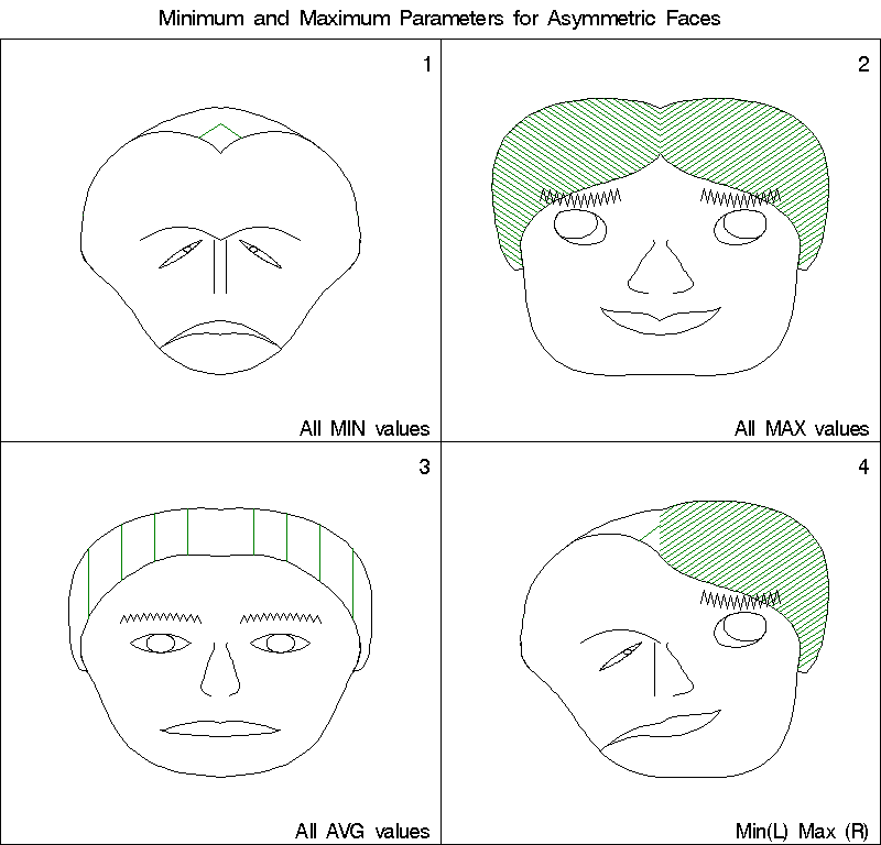
The following example creates a data set with 4 observations corresponding to the combinations of minimum (0), maximum (1) and average values on all varibles, and displays them in a faces plot.

data minmax;
   input nr r1-r18 #2 l1-l18 numid $char16.;
   r=int(nr/10);
   c=mod(nr,10);
cards;
11 0. 0. 0. 0. 0. 0. 0. 0. 0. 0. 0. 0. 0. 0. 0. 0. 0. 0.
   0. 0. 0. 0. 0. 0. 0. 0. 0. 0. 0. 0. 0. 0. 0. 0. 0. 0. All MIN values
13 1. 1. 1. 1. 1. 1. 1. 1. 1. 1. 1. 1. 1. 1. 1. 1. 1. 1.
   1. 1. 1. 1. 1. 1. 1. 1. 1. 1. 1. 1. 1. 1. 1. 1. 1. 1. All MAX values
31 .5 .5 .5 .5 .5 .5 .5 .5 .5 .5 .5 .5 .5 .5 .5 .5 .5 .5
   .5 .5 .5 .5 .5 .5 .5 .5 .5 .5 .5 .5 .5 .5 .5 .5 .5 .5 All AVG values
33 1. 1. 1. 1. 1. 1. 1. 1. 1. 1. 1. 1. 1. 1. 1. 1. 1. 1.
   0. 0. 0. 0. 0. 0. 0. 0. 0. 0. 0. 0. 0. 0. 0. 0. 0. 0. Min(L) Max (R)
 ;
title h=1.6  'Minimum and Maximum Parameters for Asymmetric Faces';
%faces(data=minmax,
   id=numid, hcolor='GREEN',
   blks=1,rows=2,cols=2, 
   left =l1 l2 l3 l4 l5 l6 l7 l8 l9 l10 l11 l12 l13 l14 l15 l16 l17 l18,
   right=r1 r2 r3 r4 r5 r6 r7 r8 r9 r10 r11 r12 r13 r14 r15 r16 r17 r18
   );
 
The following figure is produced:

See also

biplot Biplot display of variables and observations
outlier Robust multivariate outlier detection
scale Rescale variables to a given range
scatmat Scatterplot matrix
stars Star plot for multivariate data