SAS Macro Programs: heplot

The heplot macro ( get heplot.sas)

Plot Hypothesis and Error matrices for a bivariate MANOVA effect

Typically, you perform a MANOVA analysis with PROC GLM, and save the output statistics, including the H and E matrices, using the OUTSTAT= option. This must be supplied to the macro as the value of the STAT= parameter. If you also supply the raw data for the analysis via the DATA= parameter, the means for the levels of the EFFECT= parameter are also shown on the plot.

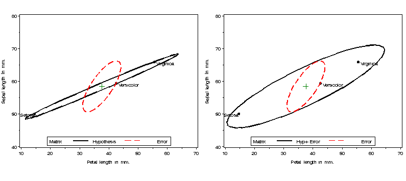
Various kinds of plots are possible, determined by the M1= and M2= parameters. The default is M1=H and M2=E. If you specify M2=I (identity matrix), then the H and E matrices are transformed to H* = eHe (where e=E^-1/2), and E*=eEe=I, so the errors become uncorrelated, and the size of H* can be judged more simply in relation to a circular E*=I. For multi-factor designs, is it sometimes useful to specify M1=H+E, so that each factor can be examined in relation to the within-cell variation.

Method

Usage

The HEPLOT macro is defined with keyword parameters. The STATS= parameter and either the VAR= or the X= and Y= parameters are required. The arguments may be listed within parentheses in any order, separated by commas. For example:

  proc glm data=dataset outstat=stats;
     model y1 y2  = A B A*B / ss3;
     manova;
  %heplot(data=dataset, stat=stats, var=y1 y2, effect=A );
  %heplot(data=dataset, stat=stats, var=y1 y2, effect=A*B );

Parameters

STAT=

Name of the OUTSTAT= dataset from proc glm containing the SSCP matrices for model effects and ERROR, as indicated by the _SOURCE_ variable.

DATA=

Name of the input, raw data dataset (for means)

X=

Name of horizontal variable for the plot

Y=

Name of vertical variable for the plot

VAR=

2 response variable names: x y. Instead of specifying X= and Y= separately, you can specify the names of two response variables with the VAR= parameter.

EFFECT=

Name of the MODEL effect to be displayed for the H matrix. This must be one of the terms on the right hand side of the MODEL statement used in the PROC GLM or PROC REG step, in the same format that this efffect is labeled in the STAT= dataset. This must be one of the values of the _SOURCE_ variable contained in the STAT= dataset.

CLASS=

Names of class variables(s), used to find the means for groups to be displayed in the plot. The default value is the value specified for effect, except that '*' characters are changed to spaces.

EFFLAB=

Label (up to 16 characters) for the H effect, annotated near the max/min corner of the H ellipse. [Default: EFFLAB=&EFFECT]

EFFLOC=

Location for the effect label: MAX (above) or MIN (below).[Default: EFFLOC=MAX]

MPLOT=

Matrices to plot [Default: MPLOT=1 2]

GPFMT=

Format for levels of the group/effect variable used in labeling group means.

ALPHA=

Non-coverage proportion for the ellipses [Default: ALPHA=0.32]

PVALUE=

Coverage proportion, 1-alpha [Default: PVALUE=0.68]

SS=

Type of SS to extract from the STAT= dataset. The possibilities are SS1-SS4, or CONTRAST (but the SSn option on the MODEL statement in PROC GLM will limit the types of SSCP matrices produced). This is the value of the _TYPE_ variable in the STAT= dataset. [Default: SS=SS3]

WHERE=

To subset both the STAT= and DATA= datasets

ANNO=

Name of an input annotate data set, used to add additional information to the plot of y * x.

ADD=

Specify ADD=CANVEC to add canonical vectors to the plot. The PROC GLM step must have included the option CANONICAL on the MANOVA statement.

M1=

First matrix: either H or H+E [Default: M1=H]

M2=

Second matrix either E or I [Default: M2=E]

SCALE=

Scale factors for M1 and M2. This can be a pair of numeric values or expressions using any of the scalar values calculated in the PROC IML step. The default scaling [SCALE=1 1] results in a plot of E/dfe and H/dfe, where the size and orientation of E shows error variation on the data scale, and H is scaled conformably, allowing the group means to be shown on the same scale. The _natural scaling_ of H and E as generalized mean squares would be H/dfh and E/dfe, which is obtained using SCALE=dfe/dfh 1. Equivalently, the E matrix can be shrunk by the same factor by specifying SCALE=1 dfh/dfe.

VAXIS=

Name of an axis statement for the y variable

HAXIS=

Name of an axis statement for the x variable

LEGEND=

Name of a LEGEND statement. If not specified, a legend for the M1 annd M2 matrices is drawn beneath the plot. Use LEGEND=NONE to suppress the legend.

COLORS=

Colors for the H and E ellipses [Default: COLORS=BLACK RED]

LINES=

Line styles for the H and E ellipses [Default: LINES=1 21]

WIDTH=

Line widths for the H and E ellipses [Default: WIDTH=3 2]

HTEXT=

Height of text in the plot. If not specified, the global graphics option HTEXT controls this.

OUT=

Name of the output dataset [Default: OUT=OUT]

NAME=

Name of the graphic catalog entry [Default: NAME=HEPLOT]

GOUT=

Name of the graphic catalog [Default: GOUT=GSEG]

Example

%include macros(heplot);        *-- or include in an autocall library;
%include data(iris);
title;
proc glm data=iris outstat=stats noprint;
   class species;
   model SepalLen sepalwid PetalLen petalwid = species / nouni ss3;
   manova h=species;
   run;

%gdispla(OFF);
axis1 label=(a=90) order=(40 to 80 by 10);
legend1 position=(bottom center inside) offset=(0,1) mode=share frame;
%heplot(data=iris,stat=stats, var=Petallen SepalLen, effect=species, 
	vaxis=axis1, legend=legend1, hsym=1.6);

%heplot(data=iris,stat=stats, var=PetalLen SepalLen, effect=species,
	vaxis=axis1,m1=H+E, legend=legend1, hsym=1.6);

%gdispla(ON);
%panels(rows=1, cols=2);

Canonical HE plots

*-- use canplot for side effect of getting Can scores and annotate dataset;
%canplot(
  data=iris,
  class=species,
  var=SepalLen SepalWid PetalLen PetalWid,
  plot=NO,
  scale=3.5);

*-- remove species circles and means from annotate data set;
data _danno_;
	set _danno_;
	where comment not in ('MEAN', 'CIRCLE');
	run;
*-- Get H and E matrices for canonical scores;
proc glm data=_dscore_ outstat=stats;
	class species;
	model can1 can2  = species / nouni ss3;
	manova h=species;
	run;

axis1 length=2.6 IN order=(-4 to 4 by 2) label=(a=90);
axis2 length=6.5 IN order=(-10 to 10 by 2);
legend1 position=(bottom center inside) offset=(0,1) mode=share frame;

%heplot(data=_dscore_, stat=stats, x=Can1, y=Can2
	,effect=species
	,haxis=axis2, vaxis=axis1, legend=none, hsym=1.6
	,anno=_danno_
);

See also