SAS Macro Programs: inflplot

The inflplot macro ( get inflplot.sas)

Influence plots for regression models

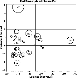
The INFLPLOT macro produces a variety of influence plots for a regression model -- plots of studentized residuals vs. leverage (hat-value), using an influence measure (COOK's D, DFFITS, COVRATIO) as the size of a bubble symbol. The plot show the components of influence (residual and leverage) as well as their combined effect.

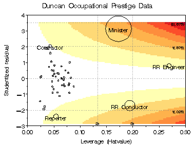
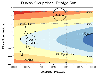
Plots can be produced either as bubble plots with PROC GPLOT or GCONTOUR plots of any of the influence measures overlaid with bubble symbols. The contour plots show how the influence measures vary with residual and leverage. Horizontal reference lines in the plots delimit observations whose studentized residuals are individually or jointly (with a Bonferonni correction) significant. Vertical reference lines in the plot shows observations which are of "high leverage".

Usage

The INFLPLOT macro is defined with keyword parameters. The Y= and X= parameters are required. The arguments may be listed within parentheses in any order, separated by commas. For example:

  %inflplot(Y=response, X=X1 X2 X3 X4, ...);

Parameters

DATA=

The name of the input data set [Default: DATA=_LAST_]

Y=

Name of the criterion variable.

X=

Names of the predictors in the model. Must be a blank-separated list of variable names.

ID=

The name of an observation ID variable. If not specified, observations are labeled sequentially, 1, 2, ...

BUBBLE=

Influence measure shown by the bubble size. Specify one of COOKD, DFFITS, or COVRATIO [Default: BUBBLE=COOKD]

CONTOUR=

Specifies influence measures shown as contours in the plot(s). One or more of COOKD, DFFITS, or COVRATIO.

LABEL=

Points to label with the value of the ID variable in the plot: One of ALL, NONE or INFL. The choice INFL causes only influential points to be labelled. [Default: LABEL=INFL]

INFL=

Criterion for declaring an influential observation, a logical expression using any of the variables in the output OUT= data set of regression diagnostics. The default is

             INFL=%STR(ABS(RSTUDENT) > TCRIT
               OR HATVALUE > HCRIT
               OR ABS(&BUBBLE)  > BCRIT)

LSIZE=

Observation label size. The height of other text is controlled by the HTEXT= goption. [Default: LSIZE=1.5]

LCOLOR=

Observation label color [Default: LCOLOR=BLACK]

LPOS=

Observation label position, using a position value understood by the Annotate facility. [Default: LPOS=5]

LFONT=

Font used for observation labels.

BSIZE=

Bubble size scale factor [Default: BSIZE=10]

BSCALE=

Scale for the bubble size. BSCALE=AREA makes the bubble area proportional to the influence measure; BSCALE=RADIUS makes the bubble radius proportional to influence. [Default: BSCALE=AREA]

BCOLOR=

Bubble color [Default: BCOLOR=RED]

BFILL=

Bubble fill? Options are BFILL=SOLID | GRADIENT , where the latter uses a gradient version of BCOLOR

HREF=

Locations of horizontal reference lines. The macro variables HCRIT and HCRIT1 are internally calculated as 2 and 3 times the average HAT value. [Default: HREF=&HCRIT &HCRIT1]

VREF=

Locations of vertical reference lines. The program computes critical values of the t-statistic for an individual residual (TCRIT) or for all residuals using a Bonferroni correction (TCRIT1) [Default: VREF=-&TCRIT1 -&TCRIT 0 &TCRIT &TCRIT1]

REFCOL=

Color of reference lines [Default: REFCOL=BLACK]

REFLIN=

Line style for reference lines. Use 0 to suppress. [Default: REFLIN=33]

GPLOT=

Whether to draw the plot using PROC GPLOT, Y or N. This may be useful if you use the CONTOUR= option and want to suppress the GPLOT version.

OUT=

The name of the output data set containing regression diagnostics [Default: OUT=_DIAG_]

OUTANNO=

Output data set containing point labels [Default: OUTANNO=_ANNO_]

NAME=

The name of the graph in the graphic catalog [Default: NAME=INFLPLOT]

GOUT=

The name of the graphics catalog

Dependencies

 %gskip Device-independent macro for multiple plots

Examples:

%include macros(inflplot);        *-- or include in an autocall library;
%include data(fuel) ;
title 'Fuel Consumption: Influence Plot';
%inflplot(data=fuel,
         y=fuel,
         x=tax drivers road inc pop,
         id=state, bsize=14);

This example shows two contour plots of Cook's D and CovRatio for the Duncan data. In both plots, bubbles are proportional to Cook's D.

 %include macros(inflplot);
 %include data(duncan) ;
 %inflplot(data=duncan,
   y=Prestige,       
   x=Income Educ,  
   id=job,
   bubble=cookd,
   bsize=14, lsize=2.5, bcolor=red,
   out=infl, outanno=labels,
   contour=cookd covratio, gplot=NO);

See also