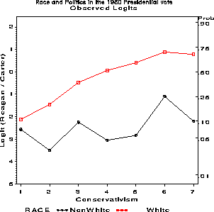
A log-linear model expresses the relationship among all variables as a model for the log of the expected cell frequency. For example, for a three-way table, the hypothesis that of no three-way association can be expressed as the log-linear model,
The log-linear model treats the variables symmetrically: none of the variables is distinguished as a response variable. However, the association parameters may be difficult to interpret, and the absence of a dependent variable makes it awkward to plot results in terms of the log-linear model. In this case, correspondence analysis and the mosaic display may provide a simpler way to display the patterns of association in a contingency table.(20)
On the other hand, if one variable can be regarded as a response or dependent variable, and the others as independent variables, then the effects of the independent variables may be expressed as a logit model. For example, if variable C is a binary response, then model (20) can be expressed as an equivalent logit model,
(21)
Both log-linear and logit models can be fit using PROC CATMOD in SAS. For logit models, the steps for fitting a model and plotting the results are similar to those used for logistic models with PROC LOGISTIC. The main differences are:
Political   ---- White ----        --- Nonwhite ---
 View      Reagan     Carter       Reagan     Carter
  1            1         12            0          6
  2           13         57            0         16
  3           44         71            2         23
  4          155        146            1         31
  5           92         61            0          8
  6          100         41            2          7
  7           18          8            0          4
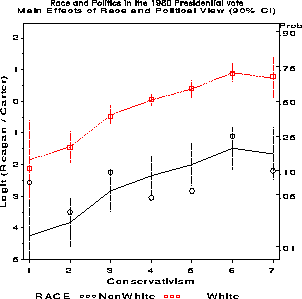
Treating the vote for Reagan vs. Carter or other as the response, a logit model with nominal main effects for race and political view is
This model does not use the ordinal nature of political view. A model which uses the value of political view as a direct, quantitative independent variable can be expressed as(22)
(23)
proc format;
  value race 0='NonWhite'
             1='White';
data vote;

  input @10 race view reagan carter;
  format race race.;
  reagan= reagan + .5;       *-- allow for 0 values;
  carter= carter + .5;
  total = reagan + carter;
  preagan = reagan / total;
  logit = log ( reagan / carter);
cards;
White    1 1    1   12
White    1 2   13   57
White    1 3   44   71
White    1 4  155  146
White    1 5   92   61
White    1 6  100   41
White    1 7   18    8
NonWhite 0 1    0    6
NonWhite 0 2    0   16
NonWhite 0 3    2   23
NonWhite 0 4    1   31
NonWhite 0 5    0    8
NonWhite 0 6    2    7
NonWhite 0 7    0    4
;
data votes;
   set vote;
   votes= reagan; votefor='REAGAN'; output;
   votes= carter; votefor='CARTER'; output;
Model (22) is fit using the statements below. The RESPONSE statement is used to produce an output data set, PREDICT, for plotting.
proc catmod data=votes order=data;
   weight votes;
   response / out=predict;
   model votefor = race view / noiter ;
   title2 f=duplex h=1.4
      'Nominal Main Effects of Race and Political View (90% CI)';
The results of the PROC CATMOD step include:
+-------------------------------------------------------------------+
|                                                                   |
|            MAXIMUM-LIKELIHOOD ANALYSIS-OF-VARIANCE TABLE          |
|                                                                   |
|          Source                   DF   Chi-Square      Prob       |
|          --------------------------------------------------       |
|          INTERCEPT                 1        43.75    0.0000       |
|          RACE                      1        41.37    0.0000       |
|          VIEW                      6        67.84    0.0000       |
|                                                                   |
|          LIKELIHOOD RATIO          6         3.45    0.7501       |
|                                                                   |
+-------------------------------------------------------------------+
+-------------------------------------------------------------------+
|                                                                   |
|              ANALYSIS OF MAXIMUM-LIKELIHOOD ESTIMATES             |
|                                                                   |
|                                     Standard    Chi-              |
|   Effect       Parameter  Estimate    Error    Square   Prob      |
|   -----------------------------------------------------------     |
|   INTERCEPT            1   -1.4324    0.2166    43.75  0.0000     |
|   RACE                 2    1.1960    0.1859    41.37  0.0000     |
|   VIEW                 3   -1.6144    0.6551     6.07  0.0137     |
|                        4   -1.2000    0.2857    17.64  0.0000     |
|                        5   -0.1997    0.2083     0.92  0.3377     |
|                        6    0.2779    0.1672     2.76  0.0965     |
|                        7    0.6291    0.1941    10.51  0.0012     |
|                        8    1.1433    0.2052    31.03  0.0000     |
|                                                                   |
+-------------------------------------------------------------------+
The data set PREDICT contains observed ( _OBS_) and predicted ( _PRED_) values, and estimated standard errors. There are 3 observations for each race-view group: logit values have _TYPE_ = 'FUNCTION'; probabilities have _TYPE_ = 'PROB'.
+-------------------------------------------------------------------+
|                                                                   |
|  RACE   VIEW  _TYPE_   _NUMBER_   _OBS_    _PRED_  _SEPRED_       |
|                                                                   |
|  White    1   FUNCTION     1     -2.120    -1.851     0.758       |
|  White    1   PROB         1      0.107     0.136     0.089       |
|  White    1   PROB         2      0.893     0.864     0.089       |
|  White    2   FUNCTION     1     -1.449    -1.437     0.297       |
|  White    2   PROB         1      0.190     0.192     0.046       |
|  White    2   PROB         2      0.810     0.808     0.046       |
|    ...                                                            |
|                                                                   |
+-------------------------------------------------------------------+
To plot the fitted logits, select the _TYPE_ = 'FUNCTION' observations in a data step.
data predict;
   set predict;
   if _type_ = 'FUNCTION';
A simple plot of predicted logits can then be obtained with the following PROC GPLOT step. (The plots displayed use the Annotate facility to add 90% confidence limits, calculated as _pred_ ± 1.645 _sepred_ , and a probability scale at the right as illustrated earlier.)
proc gplot data=predict;
   plot _pred_ * view = race
        / haxis=axis1 hminor=0 vaxis=axis2;
   symbol1 i=none v=+      h=1.5 c=black;
   symbol2 i=none v=square h=1.5 c=red  ;
   axis1 label=(h=1.4 'Conservativism') offset=(2);
   axis2 order=(-5 to 2) offset=(0,3)
         label=(h=1.4 a=90 'LOGIT(Reagan / Carter)');


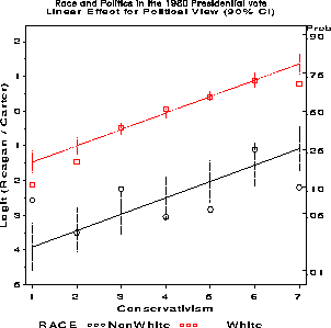
For example, to test and plot results under the assumption that political view has a linear effect on the logit scale, as in model (23), we use the same MODEL statement, but specify VIEW as a direct (quantitative) predictor.
proc catmod data=votes order=data;
   direct view;
   weight votes;
   response / out=predict;
   model votefor = race view / noiter ;
   title2 'Linear Effect for Political View (90% CI)';
   run;
The results indicate that this model fits nearly as well as the nominal main effects model, and is preferred since it is more parsimonious.
+-------------------------------------------------------------------+
|                                                                   |
|            MAXIMUM-LIKELIHOOD ANALYSIS-OF-VARIANCE TABLE          |
|                                                                   |
|          Source                   DF   Chi-Square      Prob       |
|          --------------------------------------------------       |
|          INTERCEPT                 1       101.39    0.0000       |
|          RACE                      1        42.86    0.0000       |
|          VIEW                      1        67.13    0.0000       |
|                                                                   |
|          LIKELIHOOD RATIO         11         9.58    0.5688       |
|                                                                   |
|                                                                   |
|               ANALYSIS OF MAXIMUM-LIKELIHOOD ESTIMATES            |
|                                                                   |
|                                          Standard    Chi-         |
|   Effect            Parameter  Estimate    Error    Square   Prob |
|   ----------------------------------------------------------------|
|   INTERCEPT                 1   -3.1645    0.3143   101.39  0.0000|
|   RACE                      2    1.2213    0.1865    42.86  0.0000|
|   VIEW                      3    0.4719    0.0576    67.13  0.0000|
|                                                                   |
+-------------------------------------------------------------------+
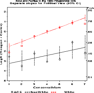
To test whether a single slope for political view, beta sup VIEW is adequate for both races, fit a model which allows separate slopes (an interaction between race and view):
proc catmod data=votes order=data;
   direct view;
   weight votes;
   response / out=predict;
   model votefor = race view race*view;
   title2 'Separate slopes for Political View (90% CI)';
The results show that this model does not offer a significant improvement in goodness of fit. The plot nevertheless indicates a slightly steeper slope for white voters than for non-white voters.
+-------------------------------------------------------------------+
|                                                                   |
|            MAXIMUM-LIKELIHOOD ANALYSIS-OF-VARIANCE TABLE          |
|                                                                   |
|          Source                   DF   Chi-Square      Prob       |
|          --------------------------------------------------       |
|          INTERCEPT                 1        26.55    0.0000       |
|          RACE                      1         2.02    0.1556       |
|          VIEW                      1         9.91    0.0016       |
|          VIEW*RACE                 1         0.78    0.3781       |
|                                                                   |
|          LIKELIHOOD RATIO         10         8.81    0.5504       |
|                                                                   |
|                                                                   |
|               ANALYSIS OF MAXIMUM-LIKELIHOOD ESTIMATES            |
|                                                                   |
|                                          Standard    Chi-         |
|   Effect            Parameter  Estimate    Error    Square   Prob |
|   ----------------------------------------------------------------|
|   INTERCEPT                 1   -2.7573    0.5351    26.55  0.0000|
|   RACE                      2    0.7599    0.5351     2.02  0.1556|
|   VIEW                      3    0.3787    0.1203     9.91  0.0016|
|   VIEW*RACE                 4    0.1060    0.1203     0.78  0.3781|
|                                                                   |
+-------------------------------------------------------------------+

