Mosaics: About Mosiac Displays

The mosaic display, proposed by Hartigan & Kleiner (1981) and extended in Friendly (1994a), represents the counts in a contingency table directly by tiles whose size is proportional to the cell frequency. This display:

generalizes readily to n-way tables
provides a method for fitting a series of sequential log-linear models to the various marginal totals of an n-way table
is used to display the deviations (residuals) from the various log-linear models.

Mosaic displays have been implemented in SAS/IML here, and also in the MANET package developed by Antony Unwin, Martin Theus and others at the University of Augsburg, in ViSta (by Forrest Young), and in a Java implementation by Martin Theus. There are rudimentary forms of mosaic displays in S-Plus (by Jay Emerson) SAS/INSIGHT and JMP software.

The new, Open Source implementation of R (www.r-project.org) now includes an object-oriented mosaicplot() on which future work will build. A newly-released R package, vcd extends mosaic displays, and implements many of the graphical methods from Visualizing Categorical Data

Two-way Tables

The construction of the mosaics display, and what it reveals, are most easily understood for two-way tables.

Consider Table 1, which shows data on the relation between hair color and eye color among 592 subjects (students in a statistics course) collected by Snee (1974). The Pearson X² for these data is 138.3 with 9 degrees of freedom, indicating substantial departure from independence. The question is how to understand the nature of the association between hair and eye color.

Table 1: Hair-color eye-color data

                      Hair Color
Eye
Color     BLACK    BROWN      RED    BLOND  | Total
                                            |
Brown        68      119       26        7  |   220
Blue         20       84       17       94  |   215
Hazel        15       54       14       10  |    93
Green         5       29       14       16  |    64
--------------------------------------------+------
Total       108      286       71      127  |   592

For such a two-way table, the mosaic display is constructed by first dividing a unit square in porportion to the marginal totals of one variable, say, Hair Color.
For these data, the marginal proportions are:
```
               Marginal proportions
        Black      Brown      Red    Blond
        0.1824    0.4831    0.1199   0.2145
```
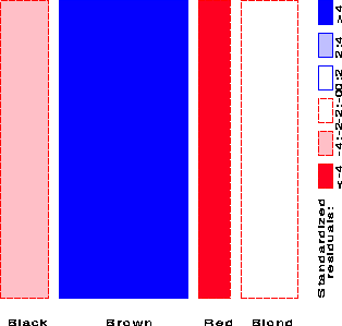
This gives the first mosaic display: The rectangular tiles are shaded to show the residuals (deviations) from a particular model, as follows:
- The one-way table of marginal totals can be fit to a model, in this case, the model that all Hair colors are equally probable. This model has expected frequencies of 592/4:
```
               Fitted frequencies
       Black      Brown      Red    Blond
       148.00    148.00    148.00   148.00
```
- The Pearson residuals from this model, d = ( n - m ) / sqrt (m), are:
```
         Standardized Pearson residuals
       Black    Brown      Red    Blond
       -3.29    11.34    -6.33    -1.73
```
  and these values are shown by color and shading as shown in the legend. The high positive value for Brown hair indicates that people with brown hair are much more frequent in the population than the Equiprobability model would predict.
Next, the rectangle for each Hair Color is subdivided in proportion to the relative (conditional) frequencies of the second variable -- Eye color, giving the following conditional proportions:
```
                     Marginal proportions
                Brown     Blue    Hazel    Green   TOTAL

      Black    0.6296   0.1852   0.1389   0.0463    1.0
      Brown    0.4161   0.2937   0.1888   0.1014    1.0
      Red      0.3662   0.2394   0.1972   0.1972    1.0
      Blond    0.0551   0.7402   0.0787   0.1260    1.0
```
This gives the second mosaic display:
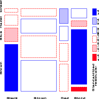
- Again, the cells are shaded in proportion to standardized residuals from a model, here, the model that Hair Color and Eye Color are independent in population from which this sample was drawn.
```
               Standardized Pearson residuals
               Brown     Blue    Hazel    Green

      Black     4.40    -3.07    -0.48    -1.95
      Brown     1.23    -1.95     1.35    -0.35
      Red      -0.07    -1.73     0.85     2.28
      Blond    -5.85     7.05    -2.23     0.61
```
- Thus, the two tiles shaded deep blue correspond to the two cells, (Black, Brown) and (Blond, Blue), whose residuals are greater than +4, indicating much greater frequency in those cells than would be found if Hair color and Eye Color were independent. The tile shaded deep red, (Blond, Brown) corresponds to the residual = -5.85, indicating this combination is extremely rare under the hypothesis of independence.
- The overall Pearson X² statistic is just the sum of squares of the residuals.

Shading levels

The default shading patterns for the tiles are based on standardized residuals which exceed the values 2 and 4 in absolute value. Since the standardized residuals are approximately unit-normal values, this corresponds to highlighting cells whose residuals are individually significant at approximately the .05 and .0001 level, respectively.

Interpretation

To interpret the association between Hair Color and Eye Color, consider the pattern of positive (Blue) and negative (Red) tiles in the mosaic display. We interpret positive values as showing cells whose observed frequency is substantially greater than would be found under independence; negative values indicate cells which occur less often than under independence.

This interpretation is enhanced by reordering the rows or columns of the two-way table so that the residuals have an opposite corner pattern of signs.

Here, this is achieved by reordering the Eye Colors as shown below:

The re-ordered residuals are:

         Standardized Pearson residuals

          Brown    Hazel    Green     Blue

Black      4.40    -0.48    -1.95    -3.07
Brown      1.23     1.35    -0.35    -1.95
Red       -0.07     0.85     2.28    -1.73
Blond     -5.85    -2.23     0.61     7.05

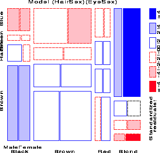
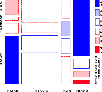
Thus, the mosaic shows that the association between Hair and Eye color is essentially that

people with dark hair tend to have dark eyes,
those with light hair tend to have light eyes
people with red hair do not quite fit this pattern

Three-way Tables

The mosaic display can be extended to three- and higher-way tables. The relative frequencies of a third variable are used to subdivide each two-way cell, and so on, recursively.

Imagine that each cell of the two-way table for Hair and Eye color is further classified by one or more additional variables--sex and level of education, for example. Then each rectangle can be subdivided horizontally to show the proportion of males and females in that cell, and each of those horizontal portions can be subdivided vertically to show the proportions of people at each educational level in the hair-eye-sex group.

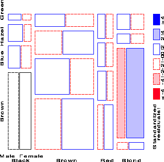
Here is the mosaic for the three-way table, with Hair and Eye color groups divided according to the proportions of Males and Females:

We see that there is no systematic association between sex and the combinations of Hair and Eye color -- except among blue-eyed blonds, where there are an overabundance of females.

Fitting models for multi-way tables

When three or more variables are represented in the mosaic, we can fit several different models of "independence" and display the residuals from that model. We treat these models as null or baseline models, which may not fit the data particularly well. The deviations of observed frequencies from expected (displayed by shading) will often suggest terms to be added to to an explanatory model which achieves a better fit.

For three-way tables, there are three different types of models of "independence" (with several instances each, permuting the variables A, B, and C):

Model	Log-linear model	Predicted cell probabilities	What the residuals show
Mutual Independence	[A] [B] [C]		Residuals show all associations among variables
Joint Independence	[A B] [C]		Residuals show associations between variable C and combinations of A and B
Conditional Independence	[A C] [ B C]	No closed-form formula	Residuals show associations between A and B, holding C constant

For higher-way tables, there are many more possibilities.

Sequential plots and models

The mosaic display is constructed in stages, with the variables listed in a given order. At each stage, the procedure fits a (sub)model to the marginal subtable defined by summing over all variables not yet entered. The series of plots can give greater insight into the relationships among all the variables than a single plot alone.

Moreover, the series of mosaic plots fitting submodels of Joint Independence to the marginal subtables have the special property that they can be viewed as partitioning the hypothesis of Mutual Independence in the full table.

For example, for the hair-eye data, the mosaic displays for the [Hair] [Eye] marginal table and the [HairEye] [Sex] table can be viewed as representing the partition

Model                      df        G²

[Hair] [Eye]                9       146.44
[Hair, Eye] [Sex]          15        19.86
------------------------------------------
[Hair] [Eye] [Sex]         24       155.20

This partitioning scheme extends directly to higher-way tables.

Marginal Subtables and Simpson's Paradox

The sequential plots of margnal subtables assume that the (unconditional) relationship among earlier variables in the ordering, ignoring later variables, is the same as the (conditional) relationship among these variables controlling for later ones. For example, we assume that Hair color and Eye color have the same relation in the marginal subtable as they do in the subtable for each sex separately.

It is possible, however, for the marginal relations among variables to differ in magnitude, or even in direction, from the relations among those variables controlling for additional variables. The peculiar result that a pair of variables can have a marginal association in a different direction than their partial associations is called Simpson's Paradox.

One way to determine if the marginal relations are representative is to fit models of Conditional Association and compare them with the marginal models. For the running example, the appropriate model is the model [Hair, Sex] [Eye, Sex], which examines the relation between Hair Color and Eye Color controlling for Sex. The fit statistic is nearly the same as for the unconditional marginal model:

Model                      df        G²

[Hair] [Eye]                9       146.44
[Hair, Sex] [Eye, Sex]     15       156.68

And, the pattern of residuals is quite similar to that of the [Hair] [Eye] marginal model, so we conclude there is no such problem here.

Animated demonstration

Imagine a survey in which people people express an opinion about their intention to vote in an upcoming election, with responses 'Yes', 'Maybe', or 'No', and we wish to see if there are differences between men and women in voting intention.

Profile differences

The animated mosaic plot below demonstrates how differences in the percentage of males in each response category appear in the mosaic display. It cycles through a series of data sets ranging from % Male = { 10, 30, 90 } to % Male = {90, 70, 10 } in a series of discrete steps.