SAS Macro Programs: hovplot

The hovplot macro ( get hovplot.sas)

Boxplot display of homogeneity of variance tests

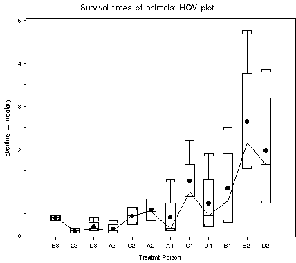
The HOVPLOT macro provides a graphical display of information related to the Levine and Brown-Forsythe tests of homogeneity of variance in factorial ANOVA designs.

Of the recommended tests of homogeneity of variance, the Levine test and the Brown-Forsythe test take simple forms amenable to graphical display. Both of these are based on an ANOVA of simple functions of a dispersion variable,

   Z  = abs (Y - median)      [Brown-Forsythe]
   Z  = abs (Y - mean)        [Levine, C<TYPE=ABS>]
   Z  =     (Y - mean)^2      [Levine, C<TYPE=SQUARE>]

O'Brien's (1979) test, is a modification of Levine's Z^2, with a more complex formula. The Brown-Forsythe test appears to have the greatest power for detecting non-constant variance.

The HOVPLOT macro displays these quantities by a set of boxplots, one for each cell in the design. Lack of homogeneity of variance is indicated by differences in spread across cells.

Method

Statistical tests are provided by PROC GLM using the HOVTEST= option on the MEANS statement, but only for one-way designs. The HOVPLOT macro extends this test to n-way designs by combining multiple CLASS= variables into a single combined variable (whose values should be distinct) representing all the cells in the design.

Usage

The HOVPLOT macro is defined with keyword parameters. The VAR= and CLASS= parameters are required. The arguments may be listed within parentheses in any order, separated by commas. For example:

  %hovplot(data=animals, var=time, class=Treatmt Poison, sortby=_iqr_);

Parameters

DATA=

Input dataset [Default: DATA=_LAST_]

WHERE=

WHERE clause to subset the data

CLASS=

Grouping variable(s)

CLASSFMT=

Format used for the CLASS= variable(s)

SEP=

Separator character used to join the values of 2 or more CLASS vars [Default: SEP=%str()]

VAR=

Name of the analysis variable

ID=

Observation ID variable, used to label extreme observations in the boxplots.

SORTBY=

How to order the classes in the boxplot. Specify the name of a dataset variable, or one of the keywords _mean_, _iqr_, _median_, etc. recognized by the BOXPLOT macro. [Default: SORTBY=]

CONNECT=

Line style to connect medians, or 0 to suppress connecting lines [Default: CONNECT=1]

NOTCH=

0 or 1, where 1 gives a notched boxplot

METHOD=

Type of HOV test: one of BF or LEVINE, LEVINE(TYPE=ABS), LEVINE(TYPE=SQUARE), or OBRIEN. Use METHOD= (null) or METHOD=NONE to suppress the numerical test. [Default: METHOD=BF]

CENTER=

Central value subtracted from Y [Default: CENTER=MEDIAN]

FUNCTION=

Function of (Y-&center) plotted, either ABS or SQUARE [Default: FUNCTION=ABS]

OUT=

Name of output dataset, a copy of the input dataset, containing additional variables _CLASS_, MEDIAN, MEAN, N

NAME=

Name for graphic catalog entry [Default: NAME=HOVPLOT]

GOUT=

The name of the graphics catalog [Default: GOUT=GSEG]

Dependencies

Requires:
boxplot
combine

Example

data animals;
   do poison=1 to 3;
      do rep = 1 to 4;
         do treatmt='A', 'B', 'C', 'D';
               group = treatmt || put(poison,1.);
            input time @;
            time = time*10;
            output;
            end;
      end;
   end;
   label treatmt='Treatment' time='Survival time (hrs)'
        poison='Poison';
datalines;
0.31  0.82  0.43  0.45
0.45  1.10  0.45  0.71
0.46  0.88  0.63  0.66
0.43  0.72  0.76  0.62
0.36  0.92  0.44  0.56
0.29  0.61  0.35  1.02
0.40  0.49  0.31  0.71
0.23  1.24  0.40  0.38
0.22  0.30  0.23  0.30
0.21  0.37  0.25  0.36
0.18  0.38  0.24  0.31
0.23  0.29  0.22  0.33

%include macros(hovplot);        *-- or include in an autocall library;

title 'Survival times of animals: HOV plot';
%hovplot(data=animals, var=time, class=Treatmt Poison, sortby=_iqr_);

See also