Visualizing Categorical Data: inflglim

The inflglim macro ( get inflglim.sas)

Influence plots for generalized linear models

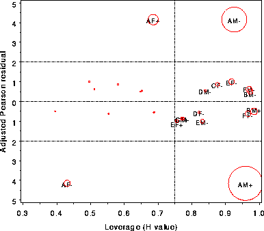
The INFLGLIM macro produces various influence plots for a generalized linear model fit by PROC GENMOD. Each of these is a bubble plot of one diagnostic measure (specified by the GY= parameter) against another (GX=), with the bubble size proportional to a measure of influence (usually, BUBBLE=COOKD). One plot is produced for each combination of the GY= and GX= parameters.

Usage

The macro normally takes an input data set of raw data and fits the GLM specified by the RESP=, and MODEL= parameters, using an error distribution given by the DIST= parameter. It fits the model, obtains the OBSTATS and PARMEST data sets, and uses these to compute some additional influence diagnostics (HAT, COOKD, DIFCHI, DIFDEV, SERES), any of which may be used as the GY= and GX= variables.

Alternatively, if you have fit a model with PROC GENMOD and saved the OBSTATS and PARMEST data sets, you may specify these with the OBSTATS= and PARMEST= parameters. The same additional diagnostics are calculated and plotted.

The INFLGLIM macro is called with keyword parameters. The MODEL= and RESP= parameters are required, and you must supply the DIST= parameter for any model with non-normal errors. The arguments may be listed within parentheses in any order, separated by commas. For example:

  %inflglim(data=berkeley,
     class=dept gender admit,
     resp=freq, model=dept|gender dept|admit,
     dist=poisson,
     id=cell,
     gx=hat, gy=streschi);

Parameters

DATA=

Name of input (raw data) data set. [Default: DATA=_LAST_]

RESP=

The name of response variable. For a loglin model, this is usually the frequency or cell count variable when the data are in grouped form (specify DIST=POISSON in this case).

MODEL=

Gives the model specification. You may use the '|' and '@' symbols to specify the model.

CLASS=

Specifies the names of any class variables used in the model.

DIST=

The name of the PROC GENMOD error distribution. If you don't specify the error distribution, PROC GENMOD uses DIST=NORMAL.

LINK=

The name of the link function. The default is the canonical link function for the error distribution given by the DIST= parameter.

OFFSET=

The name(s) of any offset variables in the model.

MOPT=

Other options on the MODEL statement (e.g., MOPT=NOINT to fit a model without an intercept).

FREQ=

The name of a frequency variable, when the data are in grouped form.

WEIGHT=

The name of an observation weight (SCWGT) variable, used, for example, to specify structural zeros in a loglin model.

ID=

Gives the name of a character observation ID variable which is used to label influential observations in the plots. Usually you will want to construct a character variable which combines the CLASS= variables into a compact cell identifier.

GY=

The names of variables in the OBSTATS data set used as ordinates for in the plot(s). One plot is produced for each combination of the words in GY by the words in GX. [Default: GY=DIFCHI STRESCHI]

GX=

Abscissa(s) for plot, usually PRED or HAT. [Default: GX=HAT]

OUT=

Name of output data set, containing the observation statistics. [Default: OUT=COOKD]

OBSTATS=

Specifies the name of the OBSTATS data set (containing residuala and other observation statistics) for a model already fitted.

PARMEST=

Specifies the name of the PARMEST data set (containing parameter estimates) for a model already fitted.

BUBBLE=

Gives the name of the variable to which the bubble size is proportional. [Default: BUBBLE=COOKD]

LABEL=

Determines which observations, if any, are labeled in the plots. If LABEL=NONE, no observations are labeled; if LABEL=ALL, all are labeled; if LABEL=INFL, only possibly influential points are labeled, as determined by the INFL= parameter. [Default: LABEL=INFL]

INFL=

Specifies the criterion used to determine which observations are influential (when used with LABEL=INFL). [Default: INFL=%STR(DIFCHI > 4 OR HAT > &HCRIT OR &BUBBLE > 1)]

LSIZE=

Observation label size. [Default: LSIZE=1.5]. The height of other text (e.g., axis labels) is controlled by the HTEXT= goption.

LCOLOR=

Observation label color. [Default: LCOLOR=BLACK]

LPOS=

Observation label position, relative to the point. [Default: LPOS=5]

LFONT=

Font used for observation labels.

BSIZE=

Bubble size scale factor. [Default: BSIZE=10]

BSCALE=

Specifies whether the bubble size is proportional to AREA or RADIUS. [Default: BSCALE=AREA]

BCOLOR=

The color of the bubble symbol. [Default: BCOLOR=RED]

BFILL=

Bubble fill? Options are BFILL=SOLID | GRADIENT, where the latter uses a gradient version of BCOLOR

REFCOL=

Color of reference lines. Reference lines are drawn at nominally 'large' values for HAT values, standardized residuals, and change in chi square values. [Default: REFCOL=BLACK]

REFLIN=

Line style for reference lines. Use REFLIN=0 to suppress these reference lines. [Default: REFLIN=33]

NAME=

Name of the graph in the graphic catalog [Default: NAME=INFLGLIM]

GOUT=

Name of the graphics catalog.

Example

%include vcd(inflglim);        *-- or include in an autocall library;
%include data(berkeley);

%inflglim(data=berkeley, class=dept gender admit,
        resp=freq, model=dept|gender dept|admit, dist=poisson, id=cell,
        gx=hat, gy=streschi);

See also