| robcov |
Calculate robust covariance matrix via MCD or MVE |
robcov |
SAS Macro Programs: robcov
$Version: 1.2 (24 Feb 2002)
Michael Friendly
York University
Calculate robust covariance matrix via MCD or MVE
The ROBCOV macro calculates robust estimates of the mean vector,
variance-covariance matrix and/or correlation matrix for a multivariate
sample. It also calculates classical estimates of multivariate
(Mahalanobis) distance, and robust estimates of multivariate distance which
ignore potential outliers. Optionally, it produces a plot of robust vs.
classical distances.
These results may be used both to detect multivariate outliers and leverage
points, and to provide robust versions of any multivariate technique which
depends on the covariance or correlation matrix, simply by substituting the
robust result for the classical ones. Typical applications include
regression, canonical correlation, factor analysis, and structural equation
models, when the input may be supplied as a covariance (correlation)
matrix, *or* when the procedure ignores observations with WEIGHT=0 to be excluded.
Two types of highly-robust estimators are provided: the minimum covariance
determinant (MCD) estimator, based on the fast-MCD algorithm of Rousseeuw
and Van Driessen (1999), and the minimum volume ellispoid (MVE) estimator
based on earlier work by Rousseeuw (1984). MCD is defined as minimizing the
determinant of the covariance matrix computed on h points, while MVE is
defined as minimizing the volume of the p-dimensional ellipsoid containing
h points.
The macro is essentially an easily-used interface to the SAS/IML MCD and
MVE call routines. It creates a copy of the input variables augmented by
the observation distances, robust distances, and weights. It creates robust
covariance and correlation data sets in the form which may be used as input
to other SAS procedures.
The ROBCOV macro is defined with keyword parameters. There are no required
parameters, but you should include an ID= variable for more interpretable results. The arguments may be listed within
parentheses in any order, separated by commas. For example:
%robcov(data=hawkins, var=x1-x4 y, id=case);
- DATA=
-
Name of the input data set [Default:
DATA=_LAST_]
- VAR=
-
List of input variable names. You may use any of the standard SAS
abbreviations for variable lists, e.g.,
VAR=X1-X20 Y1-Y3, VAR=AGE--STORAGE, or VAR=_NUMERIC_. [Default: VAR=_NUMERIC_]
- ID=
-
Name of an observation ID variable. This variable is simply copied to the
output OUT= data set.
- METHOD=
-
Robust estimation method: MVE or MCD [Default:
METHOD=MCD]
- OPT=
-
Options for the MVE or MCD call, a list of 5 numbers controlling the
details MVE and MCD methods and printed output. See the SAS System Help
(e.g., 'MCD call') for details on opt[]. The default, OPT=, is usually
sufficient; two of these options may be specified more easily with the QUANTILE= and PRINT=
options.
- QUANTILE=
-
The quantile value of the h parameter, specified as a fraction of (n+p+1).
This value may also be specified in terms of number of observations as the
value of opt[4]. If neither QUANTILE= or opt[4] are specified, the default works out to
QUANTILE=.5 or h=(n+p+1)/2. This default has a high breakdown-bound (50%) but higher
values, up to about
QUANTILE=.75 are more efficient under milder deviations from multivariate normality.
- CORRECT=
-
Apply small sample and consistency corrections to the robust
covariance matrix and robust distances? [Default:
CORRECT=Y]
- PRINT=
-
This parameter controls the printed output from the macro, and should be
one of the following: NONE, SOME, ALL. Unless
PRINT=NONE, opt[1] is modified. [Default: PRINT=SOME]
- OUT=
-
Output data set corresponding to the input DATA= data set, with classical Mahalanobis distances (DISTANCE), robust distances
(RDIST), and observation weights (WEIGHT). [Default:
OUT=OUTDATA]
- OUTR=
-
Name for the output data set containing the robust correlation matrix, a
TYPE=CORR data set. This data set is only produced if the OUTR= name is specified; if so, the macro fiddles with opt[3]. [Default: OUTR=]
- OUTC=
-
Name for the output data set containing the robust covariance matrix.
[Default:
OUTC=OUTCOV]
- PLOT=
-
If non-blank, a plot RDIST * DISTANCE is produced, with reference lines and
case labels identifying outliers. [Default:
PLOT=RDIST]
- SUBSET=
-
A logical expression to determine which observations are labeled in the
plot. [Default: (
WEIGHT=0)]
- SYMBOL=
-
Value for point symbols in the plot. [Default:
SYMBOL=DOT]
The MCD estimator underestimates the scale of the covariance
matrix, so the robust distances are slightly too large, and
too many observations tend to be nominated
as outliers.
A scale-correction (Pison et al., 2002) has been implemented, and
seems to work well enough to make CORRECT=Y the default.
For best results with the graphic plot, you should specify appropriate
graphic options, such as HTEXT=, FTEXT=, HTITLE=, FTITLE= in a
GOPTIONS statement.
Pison, G., Van Aelst, S. & Willelms, G. (2002) "Small sample corrections
for LTS and MCD," Metrika, in press.
Rousseeuw, P. J. (1984). ``Least median of squares regression,'' JASA, 79,
871-880.
Rousseeuw, P. J. & Van Driessen, K. (1990) ``A Fast Algorithm for the
Minimum Covariance Determinant Estimator,'' Technometrics, 41, 212-223.
Examples
This example uses the artificial data from Hawkins, Bradu, and Kass (1984),
containing 75 observations on 4 variables.
The first 10 observations are "bad leverage points," seriously affecting
the regression of Y on X1-X3. The next 4 observations are "good leverage
points," with high leverage on X1-X3, but small residuals on Y.
%include macros(robcov);        *-- or include in an autocall library;

%include data(hawkins);
title 'Data from Hawkins et al.";
%robcov(data=hawkins, var=x1-x3 y, id=case, correct=N);
The default output contains the MCD results, the robust COV matrix,
and the graph of robust vs. classical distance.
See SAS Output from robcovt1.sas.
Note that two of the non-outliers are flagged with WEIGHT=0,
as a result of the underestimate of scale.
When re-run with the small sample corrections,
%robcov(data=hawkins, var=x1-x3 y, id=case);
these cases are no longer flagged, and the robust distances are smaller.
See SAS Output from robcovt2.sas.
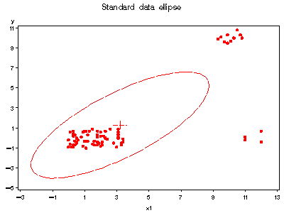
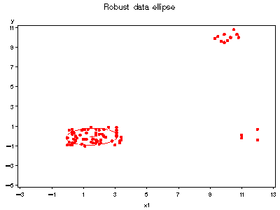
Next, get the output data set from robcov and examine data ellipses
%robcov(data=hawkins, var=x1-x3 y, id=case, out=hawkinsr);

axis1 order=(-5 to 11 by 2);
axis2 order=(-3 to 13 by 2);

title 'Standard data ellipse';
%ellipses(data=hawkinsr, y=y, x=x1, vaxis=axis1, haxis=axis2);

title 'Robust data ellipse';
%ellipses(data=hawkinsr, y=y, x=x1, weight=weight, vaxis=axis1, haxis=axis2);


See also
ellipses Plot bivariate data ellipses
outlier Robust multivariate outlier detection
robust M-estimation for robust models fitting via IRLS

