SAS Macro Programs: sprdplot
$Version: 1.2 (3 Jan 2002)
Michael Friendly
York University
Find power transformations to equalize variance
The sprdplot macro produces a spread-level plot to determine if a simple
power transformation can equalize within-group variance of a response
variable in a dataset classified by one or more classification
variables.
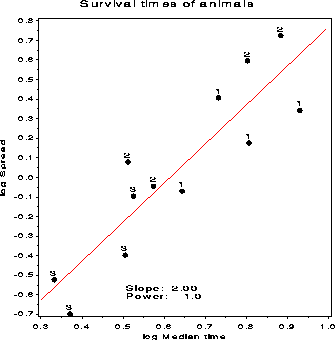
The spread-level plot has the property that *if* the relationship
between log10(Interquartile range) and log10(Median) is reasonably
linear, then the recommended power is p = 1 - slope, and the
transformation is
/ y**p, p > 0
y --> | log(p), p = 0
\ -100y**p, p < 0
The macro chooses the best power(s) from a list of simple integers
and half-integers (PLIST=), and creates new variables using those
transformations.
Method
The power is determined from the slope of a weighted linear regression
of log10(IQR) on log10(Median), using sample sizes as weights.
Usage
The SPRDPLOT macro is defined with 11 keyword parameters. The VAR= and CLASS= parameters are required. The arguments may be listed within parentheses in
any order, separated by commas. For example:
%sprdplot(data=animals, var=survive, class=treat poison);
Parameters
Default values are shown after the name of each parameter.
- DATA=
-
Name of the input dataset [Default:
DATA=_LAST_
]
- CLASS=
-
[R] Names of one or more class variables. Only the first
CLASS= variable is used as point labels in the graphics plot.
- VAR=
-
[R] Name of the variable to be transformed. Must be numeric, and should
contain all positive values.
- OFFSET=
-
Constant added to the VAR= variable before transformation. If the variable contains negative values,
OFFSET is set equal to the
abs(minimum)
value, to ensure that
all values are positive.
- PREFIX=
-
Prefix for name of transformed variable. If the PREFIX is T_ and
BEST=1
, the transformed variable is named T_&var. If BEST>1, the variables
are named T_1&var, T_2&var, ... [Default: PREFIX=T_
]
- PLIST=
-
List of powers to consider. Should be a blank-separated list of numbers in
increasing order. [Default: PLIST=-3 -2 -1 -.5 0 .5 1 2 3]
- BEST=
-
Number of best powers to transform
&var
[Default: BEST=1
]
- PPLOT=
-
Produce a printer plot? [Default:
PPLOT=N
]
- GPLOT=
-
Produce a graphics plot? [Default:
GPLOT=Y
]
- HTEXT=
-
Height of text in graphics plot [Default:
HTEXT=1.7
]
- OUT=
-
Name of the output dataset [Default: OUT=&DATA]
Example
The data give survival times (in 10 hour units) of animals exposed
to one of 3 types of poison and given one of 4 treatments, in a (3 x 4)
design, with 4 replications. Box and Cox (1964) showed that a
reciprocal transformation is reasonable.
%include macros(sprdplot); *-- or include in an autocall library;
title 'Survival times of animals';
* Hand etal #403, from Box & Cox;
data animals;
do poison=1 to 3;
do rep = 1 to 4;
do treatmt='A', 'B', 'C', 'D';
input time @;
time = time*10;
output;
end;
end;
end;
label treatmt='Treatment' time='Survival time (hrs)';
cards;
0.31 0.82 0.43 0.45 0.45 1.10 0.45 0.71
0.46 0.88 0.63 0.66 0.43 0.72 0.76 0.62
0.36 0.92 0.44 0.56 0.29 0.61 0.35 1.02
0.40 0.49 0.31 0.71 0.23 1.24 0.40 0.38
0.22 0.30 0.23 0.30 0.21 0.37 0.25 0.36
0.18 0.38 0.24 0.31 0.23 0.29 0.22 0.33
;
*-- Check for variance dependent on mean;
%sprdplot(data=animals, class=poison treatmt, var=time);
This produces the graph, chooses p= -1 (i.e., -100/Time), which is
saved in the variable T_TIME.
*-- Analyze the transformed response (T_TIME = -1/Time);
proc glm data=animals;
class poison treatmt;
model t_time = poison | treatmt;
See also
boxglm
meanplot
symplot