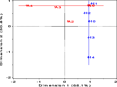
| biplot | Construct a biplot of observations and variables | biplot |
(a) A data set in table form, where the columns are separate variables and the rows are separate observations (identified by a row ID variable). In this arrangment, use the VAR= argument to specify this list of variables and the ID= variable to specify an additional variable whose values are labels for the rows.
Assume a dataset of reaction times to 4 topics in 3 experimental tasks, in a SAS dataset like this:
    TASK   TOPIC1   TOPIC2   TOPIC3   TOPIC4
    Easy     2.43     3.12     3.68     4.04
    Medium   3.41     3.91     4.07     5.10
    Hard     4.21     4.65     5.87     5.69
For this arrangment, the macro would be invoked as follows:
%biplot(var=topic1-topic4, id=task);
(b) A contingency table in frequency form (e.g., the output from PROC FREQ), or multi-way data in the univariate format used as input to PROC GLM. In this case, there will be two or more factor (class) variables, and one response variable, with one observation per cell. For this form, you must use the VAR= argument to specify the two (or more) factor (class) variables, and specify the name of response variable as the RESPONSE= parameter. Do not specify an ID= variable for this form.
For contingency table data, the response will be the cell frequency, and
you will usually use the POWER=0 parameter to perform an analysis of the log frequency.
The same data in this format would have 12 observations, and look like:
     TASK  TOPIC    RT
     Easy    1     2.43
     Easy    2     3.12
     Easy    3     3.68
     ...
     Hard    4     5.69
For this arrangment, the macro would be invoked as follows:
%biplot(var=topic task, response=RT);
In this arrangement, the order of the VAR= variables does not matter. The columns of the two-way table are determined by the variable which varies most rapidly in the input dataset (topic, in the example).
The arguments may be listed within parentheses in any order, separated by commas. For example:
%biplot(data=soccer, var=_num_, id=home);
The plot may be re-drawn or customized using the output OUT= data set of coordinates and the ANNO= Annotate data set.
The graphical representation of biplots requires that the axes in the plot are equated, so that equal distances on the ordinate and abscissa represent equal data units (to perserve distances and angles in the plot). A '+', whose vertical and horizontal lengths should be equal, is drawn at the origin to indicate whether this has been achieved.
If you do not specifiy the HAXIS= and YAXIS= parameters, the EQUATE macro is called to generate the AXIS statements to
equate the axes. In this case the INC=, XEXTRA=, and YEXTRA=, parameters may be used to control the details of the generated AXIS
statements.
By default, the macro produces and plots a two-dimensional solution.
DATA=_LAST_]
VAR=_NUM_]
DIM=2]
FACTYPE=SYM]
FACTYPE=COV: DF | N [Default: VARDEF=DF]
SCALE=1]
POWER=1]
OUT=BIPLOT]
ANNO=BIANNO]
STD=MEAN]
COLORS=BLUE RED]
SYMBOLS=NONE NONE]
INTERP=NONE VEC]
LINES=33 20]
PPLOT=NO]
PPLOT=YES. [Default: VTOH=2]
GPLOT=YES]
PLOTREQ=DIM2*DIM1]
INC=0.5 0.5]
XEXTRA=0 0]
YEXTRA=0 0]
DIMLAB=Dimension]
NAME=BIPLOT]
BIPLOT requires the following macros:
equate.sas Create AXIS statements for a GPLOT with equated axes
%include vcd(biplot);        *-- or include in an autocall library;
title 'UK Soccer scores: Biplot';
data soccer;
	input home $ a0-a4;
cards;
H0   27 29 10  8  2
H1   59 53 14 12  4
H2   28 32 14 12  4
H3   19 14  7  4  1
H4    7  8 10  2  0
;

%biplot(data=soccer, var=_num_, id=home,
	std=none, power=0,
	out=biplot, anno=bianno,
	symbols=circle dot, interp=none, inc=1);
Steps to draw the lines are omitted here.
