DataVis.ca
Michael Friendly
York University

Statistical Animations
This page collects a few examples of animated graphics used to explain statistical concepts. They mainly use the idea of plot interpolation to show a series of intermediate, interpolated views between two states of some data.They were prepared using R, with the car and heplots packages, and the animations were created with the animation package by Yihui Xie.
The headings and plots below link to individual pages with more explanation and plot controls for the animations.
Outlier detection by rotating to principal components
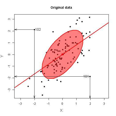 This demonstration illustrates why multivariate outliers might not be apparent
in univariate views, but become readily apparent on the smallest principal
component.
For bivariate data, principal component scores are equivalent to a rotation of the data
to a view whose coordinate axes are aligned with the major-minor axes of the data ellipse.
It is shown here by linear iterpolation between the original data, XY, and PCA scores
This demonstration illustrates why multivariate outliers might not be apparent
in univariate views, but become readily apparent on the smallest principal
component.
For bivariate data, principal component scores are equivalent to a rotation of the data
to a view whose coordinate axes are aligned with the major-minor axes of the data ellipse.
It is shown here by linear iterpolation between the original data, XY, and PCA scores
Added variable plots
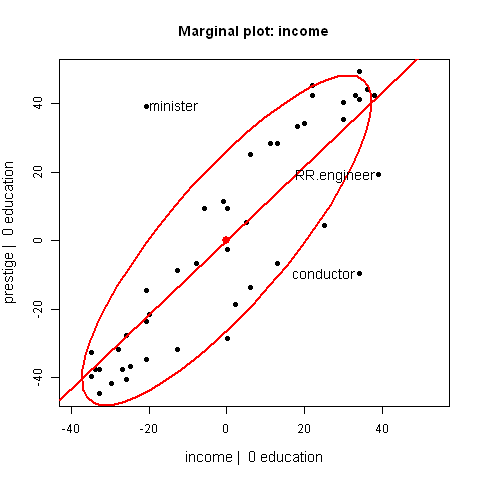 These plots show the relationship between a marginal scatterplot and an added-variable
(aka partial regression) plot by means of an animated interpolation between the
positions of points in the two plots.
They show how the slope of the regression line, the data ellipse, and positions of points
change as one goes from the marginal plot (ignoring the other variable) to the AV
plot, controlling for the other variable.
These plots show the relationship between a marginal scatterplot and an added-variable
(aka partial regression) plot by means of an animated interpolation between the
positions of points in the two plots.
They show how the slope of the regression line, the data ellipse, and positions of points
change as one goes from the marginal plot (ignoring the other variable) to the AV
plot, controlling for the other variable.
One-way MANOVA and HE plots
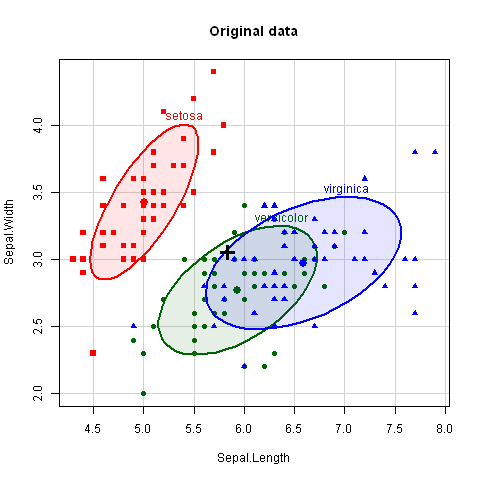 This animated series of plots illustrate the essential ideas behind the computation of
hypothesis tests in a one-way MANOVA design and how these are represented by
Hypothesis - Error (HE) plots.
This animated series of plots illustrate the essential ideas behind the computation of
hypothesis tests in a one-way MANOVA design and how these are represented by
Hypothesis - Error (HE) plots.
Bayes' Billiard Balls Experiment
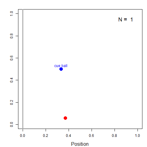
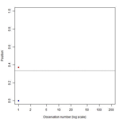 Left: Billiard table, showing average position and uncertainty;
Right: Plot of cumulative average position as more balls are thrown.
R code for animation
Thomas Bayes illustrated the thinking that led to his formulation of what is now called Bayes Theorem with the following thought experiment:
- Imagine a blue cue ball is tossed on a billiard table, but unseen by him
- How to estimate its horizontal position (0-1)?
- First guess: Ɵ=U[0,1] (prior)
- Colleague throws a red ball, reports whether it is Left or Right of the cue
- If to the right, Bayes realizes the cue ball is more likely toward the left side of the table.
- Update belief: Ɵ <0.5
- As more and more balls are thrown, each new piece of information made his imaginary cue ball wobble back and forth within a more limited area.
- Each new red ball gave more info on Ɵ
- Could use this to narrow the range of possible values for Ɵ
- Basic idea: Initial Belief + New Data -> Improved Belief.
- Now we say: Prior + likelihood -> Posterior