DataVis.ca
Michael Friendly
York University

Laurels |
|---|
 Visual Explanation
Visual explanation is about the representation of mechanism and motion, of process and dynamics, of causes and effects, of explanation and narrative. Here are a few examples.
| Picture | Words |
|---|---|

|
The Black Day: April 22, 1715 Full size (1804 x 1059; 70K).
In the early 1700s, Edmund Halley developed methods for computing the tracks of total eclipses of the sun. He determined that a total solar eclipse would sweep over southern England and Wales on Friday, April 22, 1715, the first time since 1140. He prepared a pamphlet titled The Black Day, or a prospect of Doomsday exemplified in the great and terrible eclipse which will happen on the 22nd of April 1715. He prepared this map of the predicted path of the shadow of the moon over England. But, how to describe the process that created an eclipse? Halley used the diagram at the left to show how the moon passed between the earth and sun, creating the eclipse. The letters A, B, C, D, etc. to describe their relations. C, for example, refers to the part of England predicted to be most darkened (Northhampton, 54 miles from London).
|
 |
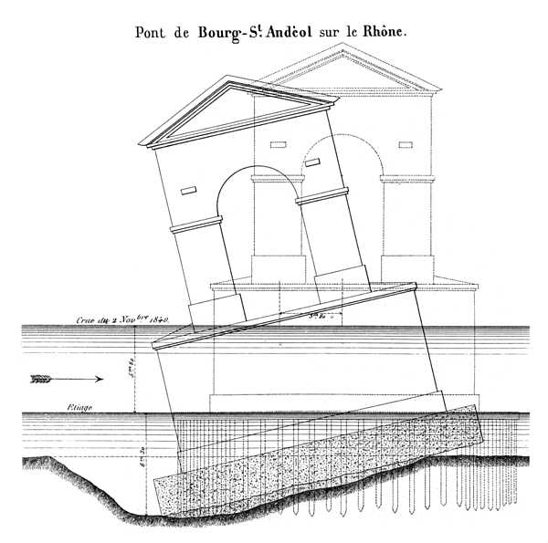
Minard as a visual engineer:
Report on the collapse of a bridge over the Rhone in 1840, medium size (335 x 335; 5.3K)
, full size (600 x 595; 36K)
Minard's main career was as an engineer for the Ecole Nationale des Ponts et Chaussees in Paris. In 1840 he was asked to investigate the cause of the collapse of the bridge at Bourg St. Andeol on the Rhone. His report consisted of this drawing, to which words provide little extra by way of explanation.
Why did the bridge collapse? As shown, the bed beneath the left side of the bridge had washed
away.
|
|
|
Visual proofs (See also the AMS page, Visual explanations in mathematics )
Proofs are usually dry, dusty stuff sprinkled liberally with symbols. What about proving something with a picture? This proof of the Pythagorean Theorem is attributed to Bhaskara, a Hindu mathematician of the 12th century. We are given the bottom right triangle. Construct a square by making three copies of the triangle, as shown. Got it? The side of the small square is b-a, and its area is (b-a)2 or b2-2ab+a2. The area of our triangle is ab/2. The area of all four triangles is 2ab. Then the area of all four triangles, plus the area of the small square is b2+a2. So c2=a2+b2. Also, see Behold! Pythagoras' Theorem for Harold Hanche-Olsen's page on this topic, which traces some of the history to the Chinese Square Proof for the (3, 4, 5) Pythagorian triple, ca. 1100 BCE, with lots of other references. |

|
Visual proofs: Jensen's Inequality
Full size (485 x 420; 38K)
Description: The essential nature of a visual proof is that the result should be immediately obvious to simple visual inspection. Beyond that, it can lead one to think about generalizations, edge cases or counter-examples, that may not be as apparent in formal mathematics. Here is an example, from Mark Reid's Behold! Jensen's Inequality, showing a proof of Jensen's Inequality, with some discussion of the relation between visual and mathematical proofs. It states that the expected value of a convex transformation, f(x), of a random variable, x, is at least the value of the convex function at the mean of the random variable, or, in symbols: E[f(x)] ≥ f(E[x]). In the diagram, E[x] is the expected value (average) of x, and f(E[x]) is the function value at that point. But the expected value, E[f(x)], of the function (over all x), must clearly lie above that, in the blue shaded region.
|
 |
Paradoxes in Regression: Suppression:
Varieties of suppression effects in multiple regression full size (562 x 417; 6.6K)
Classical suppression refers to the paradoxical result that a predictor variable (X1) may have no correlation with an outcome variable (Y), yet it increases the variance accounted for (R2) in a multiple regression with another predictor (X2). A variety of other paradoxical effects (enhancement, redundancy) can also occur, depending on the correlations among these variables. This diagram, by Friedman and Wall (2005), puts all these effects in context. It shows the regression coefficients and R2 for particular values of the correlations of Y with X1 and X2, as the correlation r12 between X1 and X2 varies over its range. The regions in which various effects occur are demarked by vertical lines. Reference: Friedman, L. and Wall, M. (2005), Graphical views of suppression and multicolinearity in multiple linear regression, The American Statistician, 59(2), 127-136. |
 |
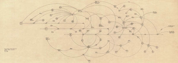
Mark Lombardi: Network Diagrams of Conspiracy:
George W. Bush, Harken Energy and Jackson Stephens
c. 1979-90, 5th Version
1999 full size (214 x 600; 16kb)
Mark Lombardi (1955-2000) was an abstract painter, best known for his network diagrams of crime and conspiracy. Lombardi's drawings attempt to document financial and political frauds by power brokers. Nodes in the diagrams represent individuals, corporations and government agencies, connected by lines showing associations, deals and so forth. His 1999 drawing, entitled George W. Bush, Harken Energy and Jackson Stephens, ca 1979-90, shows the proven connections between James Bath, the Bush and bin Laden families, and business deals in Texas and around the world. Thirteen lines originate with or point to James R. Bath, more than any other name presented. Among those linked to this obscure yet central character are George W. Bush, Jr., George H.W. Bush, Sr., Senator Lloyd Bentsen of Texas, Governor John B. Connally of Texas, Sheik Salim bin Laden of Saudi Arabia, and Sheik Salim's younger brother, Osama bin Laden. Lombardi's other network diagrams relate to the Iran-Contra Affair, World Finance Corporation, the Bay of Pigs invasion, and so forth. Each was based on thousands of notes gathered from news reports and written on index cards. See also: Review of George W. Bush, Harken Energy and Jackson Stephens for the complete story behind this image. Notes on Mark Lombardi from ArtCritical.com. [Credits:
Thanks to Daniel Seiberling for bringing Lombardi's work to my attention.]
|
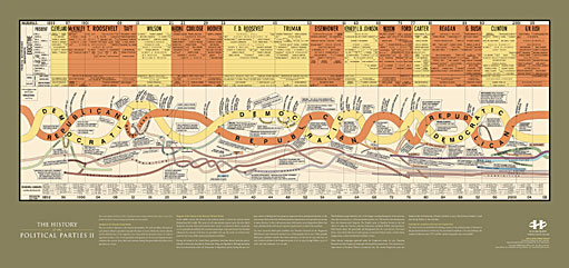 ") |
HistoryShots: Graphic depictions of events in time
Full image, medium size (511 x 241; 45K);
Full image, large (792 x 374; 164K);
Detail1 (541 x 300; 76K)
Detail2 (541 x 200; 52K)
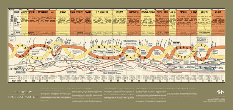
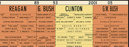
Description: Telling stories of history in words provides for rich detail, analysis, and subtlety, but the linear form of text does not provide for overview, multiple layers or zoomable levels of detail -- abstraction that might be possible in a visual representation. These images are from one of a series of beaautifully designed, poster-size charts prepared by Larry Gormley and Bill Younker of HistoryShots. This one shows the history of the US political parties from 1892--2005, on a horizontal time scale with details about political events, issues and administrations.
[Credits:
These images are Copyright © 2006 HistoryShots, LLC. All rights reserved;
used here by permission.]
|
 ") |
HistoryShots: History of the Confederate Army
Full image, medium size (527 x 354; 64K);
Detail1 (485 x 299; 65K)
Description: These images, also from HistoryShots, provide a visual analysis of the Confederate Army in the US Civil War. The main organization is by date (horizontal) and by geography (vertical). Flow lines, chart the size of armies over time, and many details of important battles are shown as annotations. Questions: How can such visual portrayals of events in time be made better or more useful? Are there better ways of representing time than a linear scale? How can other dimension(s) be used? What can be done with dynamic, interactive graphics that can't be shown in a static image? See our page on Timelines and Visual Histories for a gallery of timeline visualizations, and A Timeline of Timelines for a history of ideas about representations of time. [Credits:
These images are Copyright © 2006 HistoryShots, LLC. All rights reserved;
used here by permission.]
|
|
Animated statistical graphics: Added-variable plots
AV plot for income (480 x 480; 64K);
AV plot for education (480 x 480; 64K); See the
duncanAV page for a description of these plots.
Description: Animated graphics can be used to demonstrate or explain statistical concepts more easily than one can do in static graphs. The plot shown here illustrates the relationship between an ordinary (marginal) scatterplot that ignores other possible predictors, and a conditional, added-variable plot that controls for other variables. We can see how the slope of the regression line, the size of the data ellipse (representing precision), and the position of individual points change as on goes from the marginal relationship to the conditional one. |
|
Animated statistical graphics: MANOVA & HE plots
One-way MANOVA & HE plots (480 x 480; 236K);
See the
Animation MANOVA page for a description of these plots.
Description: Complex statistical formulas can be made more concrete by animated graphics showing the details by a series of progressive transitions. The plot shown here is an attempt at a visual explanation of the essential ideas behind multivariate analysis of variance (MANOVA) and the visualization method called HE plots. Each step in the formulas for this analysis is illustrated by a series of plot interpolations. |
