| heplot | Plot Hypothesis and Error matrices for one MLM effect | heplot |
Typically, you perform a MANOVA analysis with PROC GLM, and save
the output statistics, including the H and E matrices, using the
OUTSTAT= option. This must be supplied to the macro
as the value of the STAT=
parameter. If you also supply the raw data for the analysis via the
DATA= parameter, the means for
the levels of the EFFECT=
parameter are also shown on the plot.
Various kinds of plots are possible, determined by the M1= and M2= parameters. The default is M1=H and M2=E. If you specify M2=I (identity matrix), then the H and E matrices are transformed to H* = eHe (where e=E^-1/2), and E*=eEe=I, so the errors become uncorrelated, and the size of H* can be judged more simply in relation to a circular E*=I. For multi-factor designs, is it sometimes useful to specify M1=H+E, so that each factor can be examined in relation to the within-cell variation.
The HEPLOT macro is defined with keyword parameters. The STATS=
parameter and either the VAR= or the X= and Y= parameters are required.
The arguments may be listed within parentheses in any order, separated
by commas. For example:
  proc glm data=dataset outstat=stats;
     model y1 y2  = A B A*B / ss3;
     manova;
  %heplot(data=dataset, stat=stats, var=y1 y2, effect=A );
  %heplot(data=dataset, stat=stats, var=y1 y2, effect=A*B );
OUTSTAT= dataset from proc glm containing the
SSCP matrices for model effects and ERROR, as indicated by
the _SOURCE_ variable.
X=
and Y= separately, you can specify the names of two response
variables with the VAR= parameter.
STAT= dataset. This must be one of
the values of the _SOURCE_ variable contained in the STAT=
dataset.
EFFLOC=MAX]
MPLOT=1 2]
ALPHA=0.32]
PVALUE=0.68]
STAT= dataset. The possibilities
are SS1-SS4, or CONTRAST
(but the SSn option on the MODEL statement in
PROC GLM will limit the types of SSCP matrices produced).
This is the value of the _TYPE_ variable in the STAT= dataset.
[Default: SS=SS3]
STAT= and DATA= datasets
ADD=CANVEC to add canonical vectors to the plot. The
PROC GLM step must have included the option CANONICAL on the
MANOVA statement.
SCALE=dfe/dfh 1. Equivalently, the E matrix can
be shrunk by the same factor by specifying SCALE=1 dfh/dfe.
COLORS=BLACK RED]
LINES=1 21]
WIDTH=3 2]
OUT=OUT]
NAME=HEPLOT]
GOUT=GSEG]
%include macros(heplot);        *-- or include in an autocall library;
%include data(iris);
title;
proc glm data=iris outstat=stats noprint;
   class species;
   model SepalLen sepalwid PetalLen petalwid = species / nouni ss3;
   manova h=species;
   run;
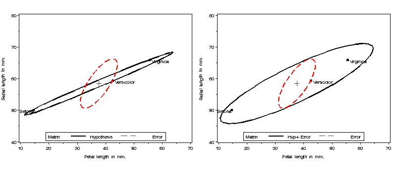
Produce two HE plots: one of H and E, and the other of (H+E) and E, for the effect of species. The VAXIS=AXIS1 parameter ensures that both plots have the same vertical axis scaling.
%gdispla(OFF);
axis1 label=(a=90) order=(40 to 80 by 10);
legend1 position=(bottom center inside) offset=(0,1) mode=share frame;
%heplot(data=iris,stat=stats, var=Petallen SepalLen, effect=species,
	vaxis=axis1, legend=legend1, hsym=1.6);

%heplot(data=iris,stat=stats, var=PetalLen SepalLen, effect=species,
	vaxis=axis1,m1=H+E, legend=legend1, hsym=1.6);

%gdispla(ON);
%panels(rows=1, cols=2);

*-- use canplot for side effect of getting Can scores and annotate dataset;
%canplot(
  data=iris,
  class=species,
  var=SepalLen SepalWid PetalLen PetalWid,
  plot=NO,
  scale=3.5);

*-- remove species circles and means from annotate data set;
data _danno_;
	set _danno_;
	where comment not in ('MEAN', 'CIRCLE');
	run;
*-- Get H and E matrices for canonical scores;
proc glm data=_dscore_ outstat=stats;
	class species;
	model can1 can2  = species / nouni ss3;
	manova h=species;
	run;

axis1 length=2.6 IN order=(-4 to 4 by 2) label=(a=90);
axis2 length=6.5 IN order=(-10 to 10 by 2);
legend1 position=(bottom center inside) offset=(0,1) mode=share frame;

%heplot(data=_dscore_, stat=stats, x=Can1, y=Can2
	,effect=species
	,haxis=axis2, vaxis=axis1, legend=none, hsym=1.6
	,anno=_danno_
);
It may be seen that the species mean-variation is essentially
one-dimensional.
